A computer program for solving the stagecoach problem/problems of Harvey Wagner [4]

A computer program for solving the stagecoach problem/problems of Harvey Wagner [4]

Jsun Yui Wong

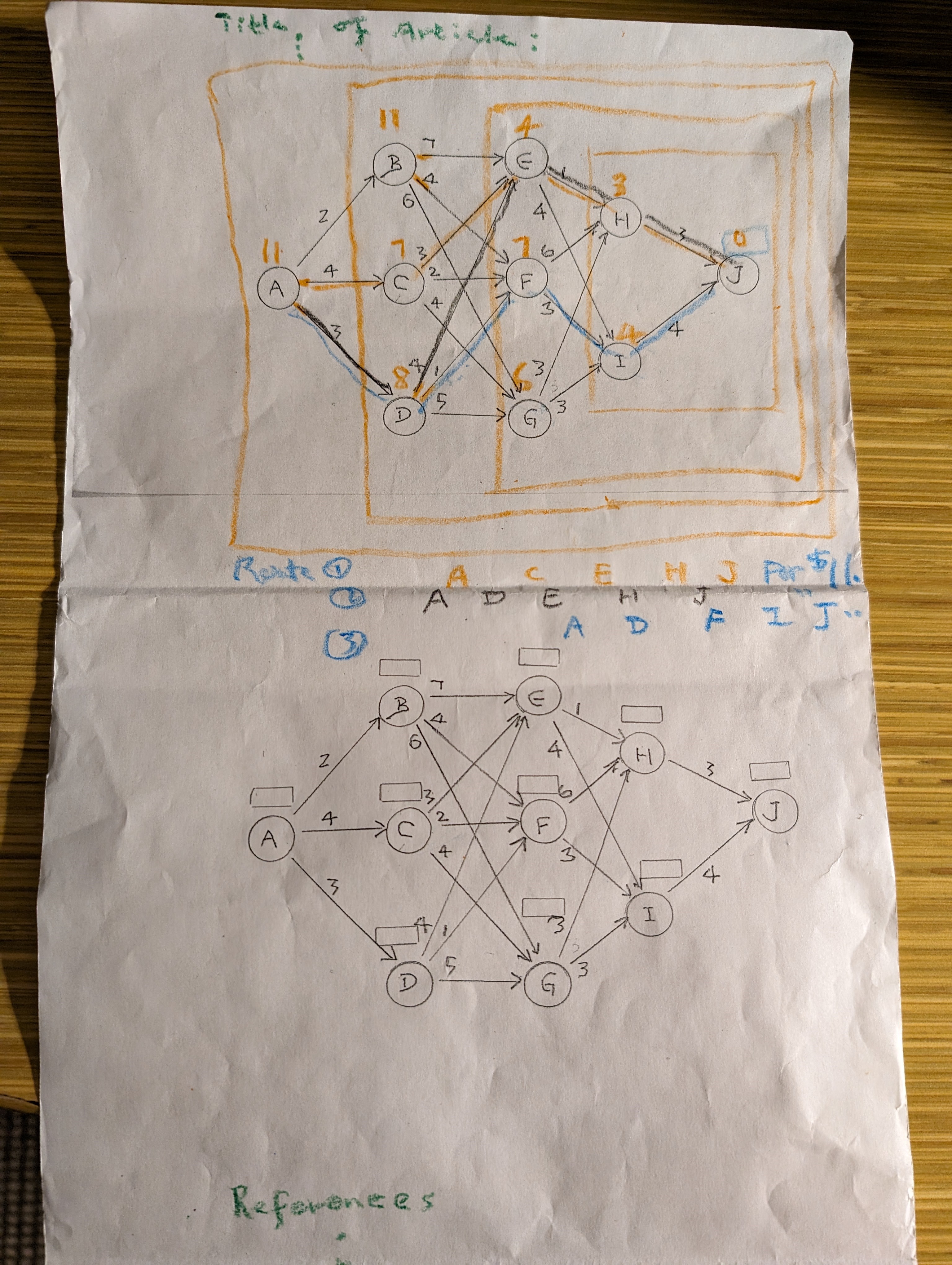
The followimg example is the stagecoach problem in Ecker and Kupferschmid [2, pp. 347-352].  Their book is available in most university libraries.  It is essential  that  one has her/his p. 348 picture to look at;  the two pictures shown below are based on their p. 348 picture, their FIGURE  10.1.  This illustration is similar to Wagner’s stagecoach problem (a prototype example for dynamic programming , [3, Hillier and Lieberman, pp. 425-430]).  All the good ideas in the present paper are from the five References listed below: Anderson et al. [1, pp. 820-829], Ecker and Kupferschmid [2 , pp. 347-352], Hillier and Lieberman [3, pp. 424-433], Wagner [4, pp.  262-270], and Wikipedia [5].

The computer program for the present example is as follows:

0 DEFINT J, K, B, X, A, N

2 DIM A(3513), X(3513), N(55)

81 FOR JJJJ = -32000 TO -31999

    89 RANDOMIZE JJJJ

    90 M = -1.5D+38

    177 N(13) = 0

    178 N(10) = 2 + 0

    179 N(11) = 4 + 0

    184 N(12) = 2 + 0

    185 N(8) = 6 + 2

    186 N(9) = 1 + 4

    187 N(5) = 4 + 5

    188 N(6) = 3 + 8

    189 N(7) = 2 + 8

    190 N(7) = 5 + 5

    192 N(2) = 3 + 9

    194 N(3) = 2 + 9

    198 N(4) = 4 + 11

    201 N(1) = 2 + 12

    1888 PRINT N(1), N(2), N(3), N(4), N(5), N(6), N(7), N(8), N(9), N(10), N(11), N(12), N(13), JJJJ

1999 NEXT JJJJ

This BASIC computer program was run with qbv1000-win [5], and the corresponding output through JJJJ=-31999 is as follows:

14   12   11   15   9

11   10   8   5   2

4   2   0   -32000

14   12   11   15   9

11   10   8   5   2

4   2   0   -31999

The wall-clock time (NOT cpu time) for producing the output above was 2 seconds when one counts from “Starting program…”.

To find the optimal path/s, one asks:  How $14 of node 1 was obtained?  Through node 2 and so on.  How $12 of node 2 obtained?  Through node 5.  How $9 of node 5 obtained?  Through node 9.  How $5 of node 9 obtained?  Through node 11.   How $4 of node 11 obtained?  Through node 13.  So path node 1-node 2-node 5-node-9- node 11-node 13 is an optimal path of 14 travel days.  This example has only one optimal route.

References

[1] D.R. Anderson, D. J. Sweeney, I. A. Williams, An introduction to management science: quantitative approaches to decision science, ninth edition, South-Western College Publishing, 2000.

[2]  J. G. Ecker, M. Kupferschmid,  Introduction to operations research, John Wiley and Sons, Inc., 1988.

[3] F. S. Hillier, G. J. Lieberman, Introduction to operations research, sixth edition, McGraw Hill, Inc.

[4] Harvey Wagner, Principles of operations research, second edition, Prentice –Hall, Inc., 1975.

[5] Wikipedia, QB64, https://en.wikipedia.org/wiki/QB64.

A fast method for solving the stagecoach problem of Harvey Wagner [4] illustrated with a prototype example for dynamic programming from Ecker and Kupferschmid [2 ]

A fast method for solving the stagecoach problem of Harvey Wagner [4] illustrated with a prototype  example for dynamic programming  from Ecker and Kupferschmid [2 ]

Jsun Yui Wong

 Here is an example like Wagner’s stagecoach problem (a prototype example for dynamic programming [3, Hillier and Lieberman], pp. 425-430).  All the good ideas in the present paper are from the five References listed below: Anderson et al. [1, pp. 820-829], Ecker and Kupferschmid [2 , pp. 347-352], Hillier and Lieberman [3, pp. 424-433], Wagner [4, pp.  262-270], and Wikipedia [5].

Please excuse this paper’s digression from the present blog. 

Today’s example is Exercise 10.4 of Ecker and Kupferschmid [2, p. 369].  Their book is available in most university libraries.  To read this paper it is necessary that one has her/his p. 369 picture (similar to picture 1 and picture 3 of the preceding paper) to look at.  The present paper depends on that.  Their example has a “directed graph with 13 nodes where the number on an arc between two nodes is the cost of using that arc in a path.  Use dynamic programming to find all minimum cost paths from node 1 to node 13,” Ecker and Kupferschmid [2, p. 369].  Then a computer program for the present example is as follows:

0 DEFINT J, K, B, X, A, N

2 DIM A(3513), X(3513), N(55)

81 FOR JJJJ = -32000 TO -31999

    89 RANDOMIZE JJJJ

    90 M = -1.5D+38

    177 N(13) = 0

    178 N(10) = 3 + 0

    179 N(11) = 2 + 0

    184 N(12) = 3 + 0

    185 N(5) = 3 + 3

    186 N(6) = 2 + 2

    189 N(7) = 1 + 3

    190 N(8) = 1 + 2

    191 N(9) = 3 + 3

    192 N(2) = 2 + 4

    193 N(3) = 2 + 4

    195 N(4) = 1 + 3

    203 N(1) = 2 + 6

    204 N(1) = 4 + 4

    1888 PRINT N(1), N(2), N(3), N(4), N(5), N(6), N(7), N(8), N(9), N(10), N(11), N(12), N(13), JJJJ

1999 NEXT JJJJ

And the corresponding output is:

8   6   6   4   6

4   4   3   6   3

2   3   0   -32000

8   6   6   4   6

4   4   3   6   3

2   3   0   -31999

The wall-clock time (not CPU time) for producing the output above was 2 seconds with counting from “Starting program…”.

To find the optimal path/s, one asks:  How $8 of node 1 was obtained?  Through node 2.  How $6 of node 2 was obtained?  Through node 6.  How $4 of node 6 was obtained?  Through node 11. How $2 of node 11 was obtained?  Through node 13. So path node 1-node 2-node 6-node-11- node 13 is an optimal path.

Also, how $8 of node 1 was obtained?  Through node 4.  How $4 of node 4 was obtained?  Through node 8. How $3 of node 8 was obtained?  Through node 11. How $2 of node 11 was obtained?  Through node 13. So path node 1-node 4-node 8-node-11- node 13 is also an optimal path.

References

[1] D.R. Anderson, D. J. Sweeney, I. A. Williams, An introduction to management science: quantitative approaches to decision science, ninth edition, South-Western College Publishing, 2000.

[2]  J. G. Ecker, M. Kupferschmid,  Introduction to operations research, John Wiley and Sons, Inc., 1988.

[3] F. S. Hillier, G. J. Lieberman, Introduction to operations research, sixth edition, McGraw Hill, Inc.

[4] Harvey Wagner, Principles of operations research, second edition, Prentice –Hall, Inc., 1975.

[5] Wikipedia, QB64, https://en.wikipedia.org/wiki/QB64.

A fast method for solving the stagecoach problem of Harvey Wagner [4] illustrated with a prototype  example for dynamic programming  from F. Hillier and G. Lieberman [3], Second Edition

Jsun Yui Wong

 Here is an illustration for solving Wagner’s stagecoach problem (a prototype example for dynamic programming [3, Hillier and Lieberman], pp. 425-430).  All the good ideas in the present paper are from the five References listed below: Anderson et al. [1, pp. 820-829], Ecker and Kupferschmid [2 , pp. 347-352], Hillier and Lieberman [3, pp. 424-433], Wagner [4, pp.  262-270], and Wikipedia [5].

Please excuse this paper’s digression from the present blog. 

Please disregard the following two pictures and the four dotes.

Please disregard the expression Title of Article: and the three dots just above the second last picture and the expression References: shown below the last picture (figure).

Please add the numbers just above the nodes of the second last picture [3, Hillier, p. 426, Figure 10.1] to the corresponding small long rectangles of the last picture.  Then the number inside each of the small rectangle above each node stands for the minimal (optimal) cost from that node to the final node, which is node 10 (note J or T), the destination.  Thus, the last two pictures show that the optimal routes are A-D-E-H-J, A-D-F-I-J, and A-C-E-H-J for the minimum total cost of 11; see Hillier and Lieberman [3, pp. 429-439].

A first step towards a computer version of the procedure above is shown below:

0 DEFINT J, K, B, X, A, N

2 DIM A(3513), X(3513), N(55)

81 FOR JJJJ = -32000 TO -31999

    89 RANDOMIZE JJJJ

    90 M = -1.5D+38

    177 N(10) = 0

    178 N(8) = 3 + 0

    179 N(9) = 4 + 0

    184 N(5) = 1 + 3

    186 N(6) = 3 + 4

    189 N(7) = 3 + 3

    192 N(2) = 4 + 7

    194 N(2) = 7 + 4

    196 N(3) = 3 + 4

    198 N(4) = 4 + 4

    199 N(4) = 1 + 7

    201 N(1) = 4 + 7

    203 N(1) = 3 + 8

    1888 PRINT N(1), N(2), N(3), N(4), N(5), N(6), N(7), N(8), N(9), N(10), JJJJ

1999 NEXT JJJJ

This BASIC computer program was run with qbv1000-win [5], and the corresponding output through JJJJ=-31999 is as follows:

11       11      7      8      4

7      6      3      4    0

-32000

11       11      7      8      4

7      6      3      4      0

-31999

The output above was obtained in one second of wall-clock time.

References

[1] D.R. Anderson, D. J. Sweeney, I. A. Williams, An introduction to management science: quantitative approaches to decision science, ninth edition, South-Western College Publishing, 2000.

[2]  J. G. Ecker, M. Kupferschmid,  Introduction to operations research, John Wiley and Sons, Inc., 1988.

[3] F. S. Hillier, G. J. Lieberman, Introduction to operations research, sixth edition, McGraw Hill, Inc.

[4] Harvey Wagner, Principles of operations research, second edition, Prentice –Hall, Inc., 1975.

[5] Wikipedia, QB64, https://en.wikipedia.org/wiki/QB64.

A fast method for solving the stagecoach problem of Harvey Wagner [4] illustrated with a prototype example for dynamic programming from F. Hillier and G. Lieberman [3]

A fast method for solving the stagecoach problem of Harvey Wagner [4] illustrated with a prototype example for dynamic programming  from F. Hillier and G. Lieberman [3]

Jsun Yui Wong

 Here is an illustration for solving Wagner’s stagecoach problem (a prototype example for dynamic programming [3, Hillier and Lieberman], pp. 425-430).  All the good ideas in the present paper are from the five References listed below: Anderson et al. [1, pp. 820-829], Ecker and Kupferschmid [2 , pp. 347-352], Hillier and Lieberman [3, pp. 424-433], Wagner [4, pp.  262-270], and Wikipedia [5].

Please excuse this paper’s digression from the present blog. 

Please disregard the following two pictures and the four dotes.

Please disregard the expression Title of Article: and the three dots just above the second last picture and the expression References: shown below the last picture (figure).

Please add the numbers just above the nodes of the second last picture [3, Hillier, p. 426, Figure 10.1] to the corresponding small long rectangles of the last picture.  Then the number inside each of the small rectangle above each node stands for the minimal (optimal) cost from that node to the final node, which is node 10 (note J or T), the destination.  Thus, the last two pictures show that the optimal routes are A-D-E-H-J, A-D-F-I-J, and A-C-E-H-J for the minimum total cost of 11; see Hillier and Lieberman [3, pp. 429-439].

A first step towards a computer version of the procedure above is shown below:

0 DEFINT J, K, B, X, A, N

2 DIM A(3513), X(3513), N(55)

81 FOR JJJJ = -32000 TO -31999

    89 RANDOMIZE JJJJ

    90 M = -1.5D+38

    177 N(10) = 0

    178 N(8) = 3 + 0

    179 N(9) = 4 + 0

    184 N(5) = 1 + 3

    186 N(6) = 3 + 4

    189 N(7) = 3 + 3

    192 N(2) = 4 + 7

    194 N(2) = 7 + 4

    196 N(3) = 3 + 4

    198 N(4) = 4 + 4

    199 N(4) = 1 + 7

    201 N(1) = 4 + 7

    203 N(1) = 3 + 8

    1888 PRINT N(1), N(2), N(3), N(4), N(5), N(6), N(7), N(8), N(9), N(10), JJJJ

1999 NEXT JJJJ

This BASIC computer program was run with qbv1000-win [5], and the corresponding output through JJJJ=-31999 is as follows:

11       11      7      8      4

7      6      3      4    0

-32000

11       11      7      8      4

7      6      3      4      0

-31999

References

[1] D.R. Anderson, D. J. Sweeney, I. A. Williams, An introduction to management science: quantitative approaches to decision science, ninth edition, South-Western College Publishing, 2000.

[2]  J. G. Ecker, M. Kupferschmid,  Introduction to operations research, John Wiley and Sons, Inc., 1988.

[3] F. S. Hillier, G. J. Lieberman, Introduction to operations research, sixth edition, McGraw Hill, Inc.

[4] Harvey Wagner, Principles of operations research, second edition, Prentice –Hall, Inc., 1975.

[5] Wikipedia, QB64, https://en.wikipedia.org/wiki/QB64.